networkx_temporal.generators

Generative models for temporal networks.

Summary - Models

dynamic_stochastic_block_model(B, z[, d, ...])	Generates a dynamic stochastic block model graph.
stochastic_block_model(B, z[, d, d_out, ...])	Generates a stochastic block model graph.

Summary - Dataset loaders

collegemsg_graph()	Returns the CollegeMsg temporal graph.
example_sbm_graph()	Returns a dynamic stochastic block model graph.
pubmed_graph([features])	Returns the PubMed temporal graph.

Summary - Utilities

community_matrix_from_vector(*community_vectors)	Converts a community vector to a community matrix.
generate_block_matrix(k[, p, q])	Generates a block matrix.
generate_community_matrix([nodes, k, ...])	Generates a node community matrix.
generate_community_vector([nodes, k, ...])	Generates a node community vector.
generate_degree_vector(nodes[, min_degree, ...])	Generates a node degree vector.
generate_transition_matrix(k[, eta, uniform_all])	Generates a transition matrix.
transition_node_memberships(communities, ...)	Simulates node-level community transitions.

dynamic_stochastic_block_model(B: List[List[float]], z: List[int], d: List[int] | None = None, d_out: List[int] | None = None, t: int | None = 1, transition_matrix: List[float] | None = None, fix_transition_prob: bool | None = False, directed: bool | None = False, multigraph: bool | None = True, isolates: bool | None = True, selfloops: bool | None = False, create_using: Graph | None = None, seed: int | None = None, sparse: bool | None = False) → TemporalGraph

Generates a dynamic stochastic block model graph. Returns a TemporalGraph object.

This model is based on a dynamic SBM model [1], where nodes are assigned to communities that may transition over time, and edges are generated based on community memberships at each snapshot. Transitions are modeled as a Markov process, where the community membership of node \(i\) at time \(t+1\), denoted by \(z^{(t+1)}_i\), depends only on its membership at time \(t\), i.e.,

\[\mathbb{P}(z_i^{(t+1)}) = \tau({z_i^{(t)}}),\]

where \(\boldsymbol{\tau}\) is the transition matrix with the same shape of the block matrix \(\mathbf{B}\). Adjacencies \(\mathbf{A}^{(t)}\) at snapshot \(t\) are sampled from a Bernoulli distribution considering the temporal communities \(\mathbf{z}^{(t)}\).

If fix_transition_prob=True, node community transition probabilities are fixed based on their initial memberships at \(t=0\) for all \(t>0\) snapshots; otherwise, considering their most recent memberships. For details on the generative model, see the stochastic_block_model() function.

Example

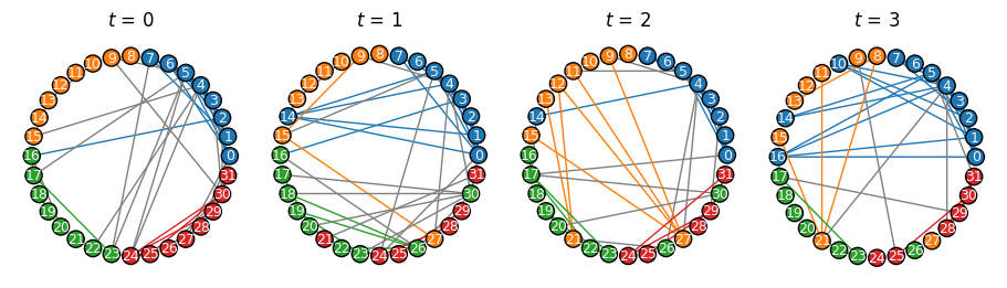
To generate a dynamic SBM with \(k=4\) communities of \(n=8\) nodes each, \(p=0.8\) within-community edge probabilities, \(t=4\) snapshots, \(\eta=0.9\) temporal community stability, and expected node degree distribution following a Zipf (power-law) with exponent \(\alpha=2\):

>>> import networkx_temporal as tx
>>>
>>> n = 8          # Nodes per community.
>>> k = 4          # Number of communities.
>>> t = 4          # Number of temporal snapshots.
>>> p = 0.8        # Within-community edge probability.
>>> eta = 0.9      # Stability of community memberships.
>>> alpha = 2      # Exponent for degree distribution (Zipf).
>>>
>>> B = tx.generators.generate_block_matrix(k, p)
>>> z = tx.generators.generate_community_vector(n, k)
>>> d = tx.generators.generate_degree_vector([n]*k, max_degree=n, alpha=alpha, seed=0)
>>> tau = tx.generators.generate_transition_matrix(k, eta)
>>>
>>> TG = tx.generators.dynamic_sbm(
>>>     B=B, z=z, d=d, t=t,
>>>     transition_matrix=tau,
>>>     fix_transition_prob=False,
>>>     seed=0
>>> )
>>> print(TG)

TemporalMultiGraph (t=4) with 32 nodes and 184 edges

Interaction times are stored in the edge attribute time. To inspect how community sizes changed over time, we may iterate over snapshots and the node attribute community:

>>> community = tx.get_node_attributes(TG, "community")
>>> for t, G in enumerate(TG):
...     clusters = [len([i for i in community[t] if i == c]) for c in set(community[t])]
...     print(f"t={t}: {G.order()} nodes, {G.size()} edges, {clusters} community sizes")

t=0: MultiDiGraph with 60 nodes and 1453 edges, [30, 30] community sizes
t=1: MultiDiGraph with 60 nodes and 1492 edges, [33, 27] community sizes

Let’s plot the resulting temporal graph, coloring nodes and edges by community memberships. We observe that few nodes transition between communities over time as \(\eta=0.9\), while most edges remain within communities and node degree distribution remains similar over time:

>>> import matplotlib.pyplot as plt
>>> colors = plt.cm.tab10.colors
>>>
>>> community = [[x for n, x in G.nodes(data="community")] for G in TG]
>>>
>>> node_color = [[colors[x] for n, x in G.nodes(data="community")] for G in TG]
>>>
>>> edge_color = [[colors[community[t][u]] if community[t][u] == community[t][v]
>>>                else "gray" for u, v in G.edges()] for t, G in enumerate(TG)]
>>>
>>> tx.draw(TG,
...         figsize=(9, 2.5),
...         layout="circular",
...         temporal_node_color=node_color,
...         temporal_edge_color=edge_color,
...         node_size=120,
...         font_size=9)

See also

The graph-tool library, which provides more efficient implementations of advanced models with features such as hierarchical community structures for large-scale networks.

[1] (1,2)

Amir Ghasemian et al. (2016). ‘’Detectability Thresholds and Optimal Algorithms for Community Structure in Dynamic Networks’’. doi: 10.1103/PhysRevX.6.031005

Parameters:

• B (List[List[float]]) – Block matrix with edge probabilities.

• z (List[int]) – Community vector assigning nodes to clusters.

• d (List[int] | None) – Vector of expected node degrees. For directed graphs, this sets the in-degree vector.

• d_out (List[int] | None) – Expected node out-degrees vector. For directed graphs, if unset, out-degrees are generated by permuting the in-degree vector. For undirected graphs, this parameter is ignored.

• t (int | None) – Number of snapshots to generate.

• transition_matrix (List[float] | None) – Transition matrix used for snapshots. If unset, nodes do not transition communities over time.

• directed (bool | None) – Whether edges are directed. Defaults to False.

• multigraph (bool | None) – Allows parallel edges. Defaults to True.

• isolates (bool | None) – Allows isolated nodes. Default is True.

• selfloops (bool | None) – Allows self-loops. Default is False.

• create_using (Graph | None) – Graph constructor to use.

• fix_transition_prob (bool | None) – If True, node transition probabilities refer to the ground truth probabilities in every snapshot. Default is False.

• seed (int | None) – Random number generator state.

• sparse (bool | None) – Whether to use sparse matrices. Default is False.

Note:

Alias to dynamic_sbm().

Return type:

TemporalGraph

stochastic_block_model(B: List[List[float]], z: List[int], d: List[int] | None = None, d_out: List[int] | None = None, directed: bool | None = False, multigraph: bool | None = True, isolates: bool | None = True, selfloops: bool | None = False, create_using: Graph | None = None, seed: int | None = None, sparse: bool | None = False) → Graph

Generates a stochastic block model graph. Returns a StaticGraph object.

Adjacencies \(\mathbf{A}\) are sampled from a Bernoulli distribution given by probabilities computed by

\[\mathbb{P}(\mathbf{A} \vert \mathbf{B}, \mathbf{z}, \mathbf{d}, \mathbf{d_{out}}) = \mathbf{\Theta_{out}} \; \mathbf{C} \; \mathbf{B} \; \mathbf{C}^\text{T} \; \mathbf{\Theta_{in}},\]

where \(\mathbf{C}\) is the \(n \times k\) community assignment matrix and \(\mathbf{\Theta}\) are diagonal matrices of degree-correction factors given by the inverse square root of the sum of expected node degrees, i.e.,

\[\theta_{in,i} = \frac{d_i}{\sqrt{\sum_{j=1}^{n} d_j}} \quad \text{and} \quad \theta_{out,i} = \frac{d_{out,i}}{\sqrt{\sum_{j=1}^{n} d_{out,j}}}.\]

If d_out=None, out-degrees are generated by permuting the in-degree vector for directed graphs; for undirected graphs, the parameter is ignored so in-degrees are equal to out-degrees.

Example

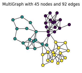
To generate an SBM with \(k=3\) communities of \(n=15\) nodes each, \(p=0.25\) within-community edge probabilities and \(q=0.01\) between-community edge probabilities:

>>> import networkx_temporal as tx
>>>
>>> k = 3
>>> n = 15
>>> p = 0.25
>>> q = 0.01
>>>
>>> B = tx.generators.generate_block_matrix(communities=k, p=p, q=q)
>>> z = tx.generators.generate_community_vector(nodes=n, communities=k)
>>> G = tx.generators.stochastic_block_model(B, z, isolates=False, seed=42)
>>>
>>> print(G)

MultiDiGraph with 45 nodes and 92 edges

>>> tx.draw(G,
>>>         figsize=(3, 3),
>>>         layout="kamada_kawai",
>>>         node_size=75,
>>>         node_color=z,
>>>         title=str(G),
>>>         with_labels=False)

See also

The graph-tool library, which provides more efficient implementations of advanced models with features such as hierarchical community structures for large-scale networks.

Parameters:

• B (List[List[float]]) – Block matrix with edge probabilities.

• z (List[int]) – Community vector assigning nodes to clusters.

• d (List[int] | None) – Vector of expected node degrees. For directed graphs, this sets the in-degree vector.

• d_out (List[int] | None) – Expected node out-degrees vector. For directed graphs, if unset, out-degrees are generated by permuting the in-degree vector. For undirected graphs, this parameter is ignored.

• directed (bool | None) – Whether edges are directed. Defaults to False.

• multigraph (bool | None) – Allows parallel edges. Defaults to True.

• isolates (bool | None) – Allows isolated nodes. Default is True.

• selfloops (bool | None) – Allows self-loops. Defaults to False.

• create_using (Graph | None) – Graph constructor to use.

• fix_transition_prob – If True, node transition probabilities refer to the ground truth probabilities in every snapshot. Default is False.

• seed (int | None) – Random number generator state.

• sparse (bool | None) – Whether to use sparse matrices. Default is False.

• note – Same as dynamic_sbm() with t=1.

Return type:

Graph

collegemsg_graph() → TemporalMultiDiGraph

Returns the CollegeMsg temporal graph.

The CollegeMsg dataset [12] is a temporal social network representing private messages sent between students at the University of California, Irvine. Nodes represent students, and a directed edge from node \(u\) to node \(v\) at time \(t\) indicates that student \(u\) sent a message to student \(v\) at time \(t\). The dataset spans 1,899 students and 59,835 messages over 193 days.

Edges have a 'time' attribute indicating the date the message was sent, following the 'YYYY-MM-DD HH:MM' format, e.g., '2002-04-05 17:30'.

Example

To load the dataset and slice() the graph into daily snapshots:

>>> import networkx_temporal as tx
>>> from datetime import datetime
>>>
>>> TG = tx.generators.collegemsg_graph()
>>>
>>> def to_date(x):
>>>     # Convert hourly dates to YYYY-MM-DD format, allowing to sort them by day.
>>>     return datetime.strptime(x.strip(), "%Y-%m-%d %H:%M").strftime("%Y-%m-%d")
>>>
>>> TG = TG.slice(attr="time", apply_func=to_date)
>>> print(TG)

TemporalMultiDiGraph (t=193) with 1899 nodes and 59835 edges

[12]

Pietro Panzarasa, Tore Opsahl, and Kathleen M. Carley. ‘’Patterns and dynamics of users’ behavior and interaction: Network analysis of an online community’’. Journal of the American Society for Information Science and Technology 60.5 (2009): 911-932. doi: 10.1002/asi.21015.

Return type:

TemporalMultiDiGraph

pubmed_graph(features: str | bool | None = False) → TemporalDiGraph

Returns the PubMed temporal graph.

The PubMed [13] temporal [14] dataset is a citation network where nodes represent scientific papers in the PubMed database, and a directed edge from node \(u\) to node \(v\) at time \(t\) indicates that paper \(u\) cited paper \(v\) at time \(t\). The dataset spans 19,717 papers and 44,335 citations over a period of 42 years, from 1967 (\(t=0\)) to 2010 (\(t=41\)). The first cited paper is from 1964.

Edges have a 'time' attribute indicating the year the citation took place, starting from 1967, while nodes have an associated 'label' attribute representing the paper’s research topic, among three possible classes If features is True, nodes will have additional attributes corresponding to the TF-IDF scores of specific words in each paper’s abstract. If the features file is not present in the specified root directory, it will be downloaded from a remote repository.

Example

To load the dataset already sliced into yearly snapshots:

>>> import networkx_temporal as tx
>>>
>>> TG = tx.generators.pubmed_graph()
>>> print(TG)

TemporalDiGraph (t=42) with 19717 nodes and 44335 edges

[13]

Namata et al. (2012). ‘’Query-driven Active Surveying for Collective Classification’’. Workshop on Mining and Learning with Graphs (MLG), Edinburgh, Scotland, UK, 2012. url: people.cs.vt.edu/~bhuang/papers/namata-mlg12.pdf.

[14]

Passos, N.A.R.A., Carlini, E., Trani, S. (2024). ‘’Deep Community Detection in Attributed Temporal Graphs: Experimental Evaluation of Current Approaches’’. In Proceedings of the 3rd GNNet Workshop: Graph Neural Networking Workshop. The 20th International Conference on emerging Networking EXperiments and Technologies (CoNEXT 2024), Los Angeles, CA, USA. doi: 10.1145/3694811.3697822.

Parameters:

features (str | bool | None) – If True, loads additional node features from file. Allows passing a string pointing to the directory where the pubmed-features.csv.gz file is located. If the file is not found, it will be downloaded automatically. Default is False.

Note:

Dataset and files available from Zenodo.

Return type:

TemporalDiGraph

example_sbm_graph() → TemporalMultiDiGraph

Returns a dynamic stochastic block model graph.

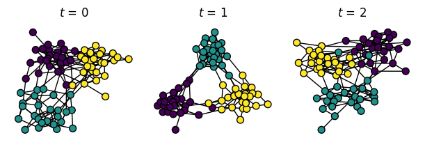
This function calls dynamic_stochastic_block_model() to create a temporal graph with 75 nodes divided into 3 communities, composed of 3 snapshots. Edges between nodes within the same community are created with a probability of 20%, or 1% among different communities. Not all nodes are guaranteed to be connected at each snapshot and isolates are removed.

Example

To load the dataset:

>>> import networkx_temporal as tx
>>>
>>> TG = tx.generators.example_sbm_graph()
>>> print(TG)

TemporalMultiDiGraph (t=3) with 75 nodes and 563 edges

Which corresponds to the graph generated with dynamic_stochastic_block_model() as follows:

>>> import networkx_temporal as tx
>>>
>>> k = 3         # Number of communities.
>>> n = 25        # Number of nodes.
>>> t = 3         # Number of snapshots.
>>> p_in = 0.2    # Probability of within-community edges.
>>> p_out = 0.01  # Probability of between-community edges.
>>>
>>> B = tx.generate_block_matrix(k, p=p_in, q=p_out)
>>> z = tx.generate_community_vector(nodes=n, k=k)
>>> TG = tx.dynamic_stochastic_block_model(B, z, t=t, isolates=False, seed=10)
>>>
>>> tx.draw(TG,
...         figsize=(6, 2),
...         layout="spring",
...         node_size=50,
...         temporal_node_color=tx.get_node_attributes(TG, "community"),
...         with_labels=False)

Return type:

TemporalMultiDiGraph

community_matrix_from_vector(*community_vectors: ndarray) → ndarray

Converts a community vector to a community matrix.

Parameters:

community_vectors (ndarray) – Community assignment vector(s) with shape (n_nodes,).

Return type:

ndarray

generate_block_matrix(k: int, p: float | None = None, q: float | None = None) → ndarray

Generates a block matrix.

A square matrix of size \(k \times k\) is generated where diagonal elements of the block matrix represent the probabilities of edges between nodes in the same community, while off-diagonal elements represent the probabilities of edges between nodes in different communities, i.e.,

\[\begin{split}\mathbf{B} = \begin{pmatrix} b_{11} & b_{12} & \cdots & b_{1k} \\ b_{21} & b_{22} & \cdots & b_{2k} \\ \vdots & \vdots & \ddots & \vdots \\ b_{k1} & b_{k2} & \cdots & b_{kk} \end{pmatrix},\, b_{ij} = \begin{cases} p & \text{if} \, i = j \\ q & \text{otherwise}. \end{cases}\end{split}\]

In this function, parameters \(p\) and \(q\) are used to set the diagonal and off-diagonal elements, respectively. If both are unset, probabilities are uniformly distributed, i.e., \(p = q = 1 / k\). If only one is unset, the other is set to \(p = 1 - q \, (k - 1)\) or \(q = (1 - p) / (k - 1)\), respectively.

Parameters:

• k (int) – Number of communities in the network.

• p (float | None) – Edge probability among nodes in the same community.

• q (float | None) – Edge probability among nodes in different communities.

Return type:

ndarray

generate_community_matrix(nodes: int | list = None, k: int | None = None, shuffle: bool | None = False, seed: int | None = None) → ndarray

Generates a node community matrix.

The community matrix is \(n \times k\) matrix that describes the community membership of each node in the graph and is used to generate the network at each time step. The community matrix is generated by repeating the community index \(i\) for each node in the community \(c\), i.e.,

\[\begin{split}\mathbf{Z} = \begin{pmatrix} z_{1,1} & z_{1,2} & \cdots & z_{1,k} \\ z_{2,1} & z_{2,2} & \cdots & z_{2,k} \\ \vdots & \vdots & \ddots & \vdots \\ z_{n,1} & z_{n,2} & \cdots & z_{n,k} \end{pmatrix},\end{split}\]

where \(\mathbf{Z}\) is the community matrix, \(z_{i,j}\) is the community index of node \(i\) in community \(j\), \(k\) is the number of communities, and \(n\) is the number of nodes in the network. Unlike in a community vector, nodes may belong to multiple communities with varying degrees of membership.

Example

>>> import networkx_temporal as tx
>>>
>>> # Generate a community matrix with 6 nodes divided into 2 communities.
>>> Z = tx.generators.generate_community_matrix(n=3, k=2, shuffle=False)
>>>
>>> print(Z)

[[1. 0.]
 [1. 0.]
 [1. 0.]
 [0. 1.]
 [0. 1.]
 [0. 1.]]

Parameters:

• nodes (int | list) – An int with the number of nodes per community or a list with the number of nodes in each community (their sizes).

• k (int | None) – Number of communities, if nodes is an int.

• shuffle (bool | None) – If True, vector elements are shuffled. Optional.

• seed (int | None) – Random seed for reproducibility. Optional.

Return type:

ndarray

generate_community_vector(nodes: int | list = None, k: int | None = None, shuffle: bool | None = False, seed: int | None = None) → ndarray

Generates a node community vector.

The community vector is a list of integers that describes the community membership of each node in the graph and is used to generate the network at each time step. The community vector is generated by repeating the community index \(i\) for each node in the community \(c\), i.e.,

\[\mathbf{z} = \big[ z_{1}, z_{2}, \cdots, z_{n} \, | \, z_{i} \leq k \big],\]

where \(\mathbf{z}\) is the community vector, \(z_{i}\) is the community index of node \(i\), \(c\) is the community index, \(k\) is the number of communities, and \(n\) is the number of nodes in the network.

Example

>>> import networkx_temporal as tx
>>>
>>> # Generate a community vector for 10 nodes for each of 2 communities.
>>> z = tx.generators.generate_community_vector(nodes=10, communities=2, shuffle=True)
>>> print(z)

[1 1 0 1 0 0 0 1 0 0 1 0 0 0 1 1 1 1 1 0]

>>> # Generate a community vector for communities of different sizes.
>>> z = tx.generators.generate_community_vector(nodes=[4, 6, 10], shuffle=False)
>>> print(z)

[0 0 0 0 1 1 1 1 1 1 2 2 2 2 2 2 2 2 2 2]

Parameters:

• nodes (int | list) – An int with the number of nodes per community or a list with the number of nodes in each community (their sizes).

• k (int | None) – Number of communities, if nodes is an int.

• shuffle (bool | None) – If True, vector elements are shuffled. Optional.

• seed (int | None) – Random seed for reproducibility. Optional.

Return type:

ndarray

generate_degree_vector(nodes: int | list, min_degree: int | None = None, max_degree: int | None = None, alpha: float | None = None, phi: float | None = None, shuffle: bool | None = True, seed: int | None = None) → ndarray

Generates a node degree vector.

The degree vector is a list of integers with the degrees of each node in the graph, which may be provided to the dynamic_sbm() generator to create graphs with expected degree distributions.

By default, if alpha and phi are unset, degrees are generated by sampling from a uniform distribution between \(d_{min}\) and \(d_{max}\), that is, \(\mathbf{d} = \big[ d_{1}, d_{2}, \cdots, d_{n} \, | \, d_{min} \leq d \leq d_{max} \big]\).

Gaussian distribution

If phi is set, the degree vector is sampled from a Gaussian (normal) distribution:

\[\mathbf{d} = \big[ d_{1}, \cdots, d_{n} \,| \, d \sim \mathcal{N} \big( \mu = \frac{d_{min} + d_{max}}{2}, \, \sigma = \frac{d_{max} - d_{min}}{\varphi} \big), \, d_{min} \leq d \leq d_{max} \big],\]

where \(\varphi \gt 0\) is a standard deviation factor that controls how it is spread around the mean \(\mu\).

Zipf distribution

If alpha is set, the degree vector is sampled from a Zipf (power-law) distribution:

\[\begin{split}\mathbf{d} = \big[ d_{1}, \cdots, d_{n} \, | \, p(d) = \frac{d^{-(\alpha + 1)}}{\sum_{d_{min}}^{d_{max}} d^{-(\alpha + 1)}}, \, d_{min} \leq d \leq d_{max} \big],\\\end{split}\]

where \(\alpha \gt 1\) is the exponent of the power-law distribution that controls how heavy-tailed it is.

Example

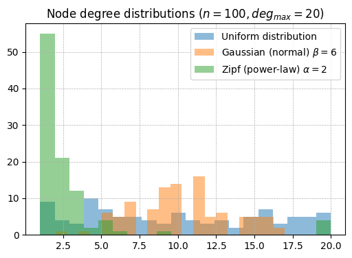
Comparison of degree distributions generated with this function:

>>> import matplotlib.pyplot as plt
>>> import networkx_temporal as tx
>>>
>>> d1 = tx.generators.generate_degree_vector(100, max_degree=20, seed=0)
>>> d2 = tx.generators.generate_degree_vector(100, max_degree=20, phi=6, seed=0)
>>> d3 = tx.generators.generate_degree_vector(100, max_degree=20, alpha=2, seed=0)
>>>
>>> fig = plt.figure(figsize=(6, 4))
>>> plt.hist(d1, bins=20, alpha=0.5, label='Uniform distribution')
>>> plt.hist(d2, bins=20, alpha=0.5, label='Gaussian (normal) $\phi=6$')
>>> plt.hist(d3, bins=20, alpha=0.5, label='Zipf (power-law) $\alpha=2$')
>>> plt.title("Node degree distributions ($n=100, deg_{max}=20$)")
>>> plt.grid("#dddddd", linestyle='--', linewidth=0.5)
>>> plt.legend()
>>> plt.show()

Parameters:

• nodes (int | list) – An int with the number of nodes in the network or a list with the number of nodes in each community (their sizes).

• min_degree (int | None) – Minimum node degree. Defaults to 1.

• max_degree (int | None) – Maximum node degree. Defaults to nodes - 1.

• alpha (float | None) – Exponent of the power-law degree distribution.

• phi (float | None) – Standard deviation factor of the normal distribution.

• shuffle (bool | None) – If True, vector elements are shuffled. Default.

• seed (int | None) – Random seed for reproducibility. Optional.

Return type:

ndarray

generate_transition_matrix(k: int, eta: float | List[float] | None = None, uniform_all: bool | None = False) → ndarray

Generates a transition matrix.

The transition matrix is a square and symmetrical matrix of size \(k \times k\) that describes the probabilities of nodes transitioning communities. The probability of a node remaining in its community is given by \(\eta\) = eta, and that of transitioning to another community by \(1 - \eta\), i.e.,

\[\begin{split}\boldsymbol{\tau} = \begin{pmatrix} \tau_{11} & \tau_{12} & \cdots & \tau_{1k} \\ \tau_{21} & \tau_{22} & \cdots & \tau_{2k} \\ \vdots & \vdots & \ddots & \vdots \\ \tau_{k1} & \tau_{k2} & \cdots & \tau_{kk} \end{pmatrix},\, \tau_{ij} = \begin{cases} \eta & \text{if} \, i = j \\ \frac{1 - \eta}{k - 1} & \text{otherwise}, \end{cases}\end{split}\]

where \(\boldsymbol{\tau}\) is the transition matrix, \(\eta \in [0, 1]\) is a parameter, and \(k\) is the number of communities, so larger values of \(\eta\) increase the probability of nodes remaining in their current community.

If eta is unset, it defaults to \(\eta = 1/k\). A list of probabilities may also be provided to define non-uniform transition probabilities for each community, e.g., eta = [0.8, 0.6, 0.9] for k=3.

Note

If uniform_all=True, uniform-at-random probabilities follow the original paper [1] and include the node’s current community in the distribution, i.e., \(\tau_{ij} = (1 - \eta)/k + \eta \, \delta(i,j)\), so nodes always have a non-zero probability of remaining in their current community even if \(\eta = 0\).

Example

>>> import networkx_temporal as tx
>>>
>>> # Generate a transition matrix for 3 communities with varying stability rates:
>>> tau = tx.generators.generate_transition_matrix(k=3, eta=[.5, .6, .8])
>>> print(tau)

array([[0.5, 0.25, 0.25],
       [0.2, 0.6 , 0.2 ],
       [0.1, 0.1,  0.8 ]])

Parameters:

• k (int) – Number of communities in the network.

• eta (float | List[float] | None) – Probability of nodes remaining in their current community. Accepts a float or a list of floats of size \(k\).

• uniform_all (bool | None) – If True, nodes remain in their current communities with an added probability \((1 - \eta)/k\). Default is False.

Return type:

ndarray

transition_node_memberships(communities: List[int] | List[List[float]], transition_matrix: List[float], seed: int | None = None) → ndarray

Simulates node-level community transitions.

The function simulates the transition of nodes between communities at time \(t+1\) based on a \(k \times k\) transition matrix \(\boldsymbol{\tau}\) = tau, where diagonals describe the probability of a node remaining in its current community and off-diagonals those of nodes switching to other communities.

Accepts either a vector (hard clustering) or a matrix (soft clustering) as communities. If a matrix, transition probabilities are computed as the dot product between the community membership strengths and the transition matrix. Returns new community assignments from transitions.

Example

Transition of mixed node memberships defined by a community matrix (soft clustering):

>>> import networkx_temporal as tx
>>>
>>> transition_matrix = [
>>>     [ 1,  0,  0],  # Nodes in the third community always remain in them.
>>>     [.2, .2, .6],  # Nodes in the second community mostly transition out.
>>>     [.5, .5,  0],  # Nodes in the third community always transition out.
>>> ]
>>> community_matrix = [
>>>     [ 1,  0,  0],  # Node in the first community.
>>>     [ 0,  1,  0],  # Node in the second community.
>>>     [ 0,  0,  1],  # Node in the third community.
>>>     [.9, .1,  0],  # Node mostly in the first community.
>>>     [.2, .6, .2],  # Node mostly in the second community.
>>>     [.5,  0, .5],  # Node equally in the first and third communities.
>>> ]
>>>
>>> new_memberships = tx.transition_node_memberships(
>>>     community_matrix,
>>>     transition_matrix=transition_matrix,
>>>     seed=0,
>>> )
>>> print(new_memberships)

[0 2 1 0 1 0]

Transition of node memberships defined by a community vector (hard clustering):

>>> # Total of 3 communities with 2 nodes each.
>>> community_vector = [0, 0, 1, 1, 2, 2]
>>>
>>> new_memberships = tx.transition_node_memberships(
>>>     community_vector,
>>>     transition_matrix=transition_matrix,
>>>     seed=0,
>>> )
>>> print(new_memberships)

[0 0 2 2 0 1]

Parameters:

• communities (List[int] | List[List[float]]) – Community assignments of nodes, either as a vector (hard clustering) or a matrix (soft clustering).

• transition_matrix (List[float]) – The transition probability matrix.

• seed (int | None) – Random seed for reproducibility. Optional.

Return type:

ndarray