See also

All examples in this guide are also available as an interactive Jupyter notebook (open on Colab).

Basic operations

The examples below cover the package’s basic functionalities, including how to build a temporal graph, slice it into snapshots, save and load graph objects to disk, and other inherited methods.

Build temporal graph

This package implements new TemporalGraph classes, which extend NetworkX graphs to handle temporal (dynamic) data. Let’s start by creating a simple directed graph using time as attribute key:

>>> import networkx_temporal as tx
>>>
>>> TG = tx.temporal_graph(directed=True)  # tx.TemporalMultiDiGraph()
>>>
>>> TG.add_edge("a", "b", time=0)
>>> TG.add_edge("c", "b", time=1)
>>> TG.add_edge("d", "c", time=2)
>>> TG.add_edge("d", "e", time=2)
>>> TG.add_edge("a", "c", time=2)
>>> TG.add_edge("f", "e", time=3)
>>> TG.add_edge("f", "a", time=3)
>>> TG.add_edge("f", "b", time=3)
>>>
>>> print(TG)

TemporalMultiDiGraph (t=1) with 6 nodes and 8 edges

Note that the resulting graph object reports a single time step t=1, as it has not yet been sliced.

Hint

To allow multiple interactions between the same nodes over time, a TemporalMultiGraph or TemporalMultiDiGraph object is required. Otherwise, only a single edge is allowed among pairs.

Import static graphs

Static graphs from NetworkX can be converted into temporal graphs with from_static():

>>> import networkx as nx
>>>
>>> G = nx.DiGraph()
>>>
>>> G.add_nodes_from([
>>>     ("a", {"time": 0}),
>>>     ("b", {"time": 0}),
>>>     ("c", {"time": 1}),
>>>     ("d", {"time": 2}),
>>>     ("e", {"time": 3}),
>>>     ("f", {"time": 3}),
>>> ])
>>>
>>> G.add_edges_from([
>>>     ("a", "b", {"time": 0}),
>>>     ("c", "b", {"time": 1}),
>>>     ("d", "c", {"time": 2}),
>>>     ("d", "e", {"time": 2}),
>>>     ("a", "c", {"time": 2}),
>>>     ("f", "e", {"time": 3}),
>>>     ("f", "a", {"time": 3}),
>>>     ("f", "b", {"time": 3}),
>>> ])
>>>
>>> TG = tx.from_static(G)
>>> print(TG)

TemporalDiGraph (t=1) with 6 nodes and 8 edges

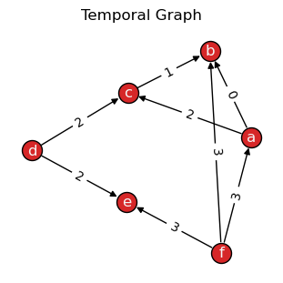
In the example above, both nodes and edges contain a time attribute, and slicing the graph using either node-level or edge-level data will yield different results. Let’s draw() the static graph:

>>> tx.draw(TG, layout="kamada_kawai", edge_labels="time", suptitle="Temporal Graph")

Slice temporal graph

Let’s use the slice() method to split the temporal graph into a number of snapshots:

>>> TG = TG.slice(attr="time")
>>> print(TG)

TemporalDiGraph (t=4) with 6 nodes and 8 edges

>>> for t, G in enumerate(TG):
>>>     print(f"Snapshot t={t}: {G.order()} nodes, {G.size()} edges")

Snapshot t=0: 2 nodes, 1 edges
Snapshot t=1: 2 nodes, 1 edges
Snapshot t=2: 4 nodes, 3 edges
Snapshot t=3: 4 nodes, 3 edges

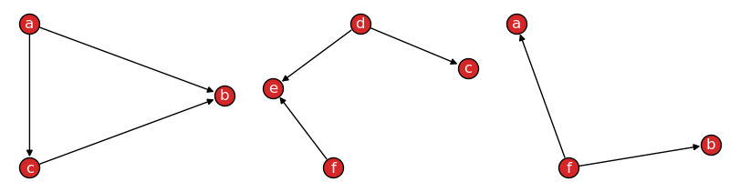
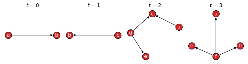
When sliced, draw() will return a plot of each resulting snapshot in the temporal graph:

>>> tx.draw(TG, layout="kamada_kawai", figsize=(8, 2))

Define number of snapshots

By default, slice() returns snapshots based on unique attribute values, here \(t \in \{0,1,2,3\}\), which are stored in the names property of TemporalGraph objects for future access.

A new object can be created with a specific number of snapshots by setting the bins parameter:

>>> TG = TG.slice(attr="time", bins=2)
>>> tx.draw(TG, layout="kamada_kawai", figsize=(4, 2), names=True)

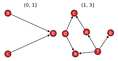
In case slice() is not able to split the graph into the specified number of bins, for example, due to insufficient data (nodes/edges), the maximum possible number of snapshots is returned instead.

Cut by snapshot order or size

Passing axis=1 to slice() will bin snapshots based on their number of nodes or edges, as defined by the level argument, optionally considering temporal information available as their attr, if set:

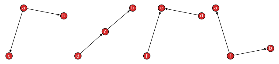
>>> TG = TG.slice(3, attr="time", axis=1)  # level="edge" (default)
>>> tx.draw(TG, layout="kamada_kawai", figsize=(8, 2), names=False)

Or, to limit the maximum number of nodes allowed per snapshot, set axis=1 and level='node':

>>> TG = TG.slice(3, axis=1, level="node")
>>> tx.draw(TG, layout="kamada_kawai", figsize=(9, 2), names=False)

Node or edge attributes

By default, the slice() function considers level="edge" attribute data:

>>> TG = TG.slice(attr="time")  # level="edge" (default)
>>> tx.draw(TG, layout="kamada_kawai", figsize=(8, 2))

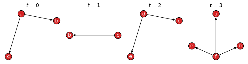
If level='node' is set, node-level attribute data is used to determine snapshots:

>>> TG_node = TG.slice(attr="time", level="node")
>>> tx.draw(TG_node, layout="kamada_kawai", figsize=(8, 2))

Quantile-based cut

Setting qcut=True slices a graph into quantiles, creating snapshots with balanced order and/or size (nodes/edges). This is useful when interactions are not evenly distributed across time. For example:

>>> TG = TG.slice(attr="time", bins=2, qcut=True)
>>> tx.draw(TG, layout="kamada_kawai", figsize=(4, 2), names=True)

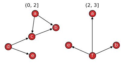
The resulting snapshots have uneven time intervals: \(t=(0,2]\) and \(t=(2,3]\), respectively. Objects are sorted by their time attribute values and then split into two groups with approximately the same order (nodes) or size (edges), depending on the level of the attribute passed to the function.

See also

The pandas.qcut documentation for more information on quantile-based discretization.

Rank-based cut

Setting rank_first=True slices a graph considering the order of appearance of edges (default), nodes, or attributes, forcing each snapshot to have approximately the same number of elements:

>>> TG = TG.slice(bins=2, rank_first=True)
>>> tx.draw(TG, layout="kamada_kawai", figsize=(4, 2), names=True)

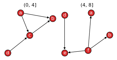
As attr was not set, the graph was split considering the order in which edges were added to the graph. Notice how each snapshot title now refer to edge intervals: \(e_0\) to \(e_3\) \((0, 4]\) and \(e_4\) to \(e_7\) \((4, 8]\). This is useful to obtain an arbitrary number of subgraphs, independent of their temporal dynamics.

See also

The pandas.rank documentation for more information on ranking data.

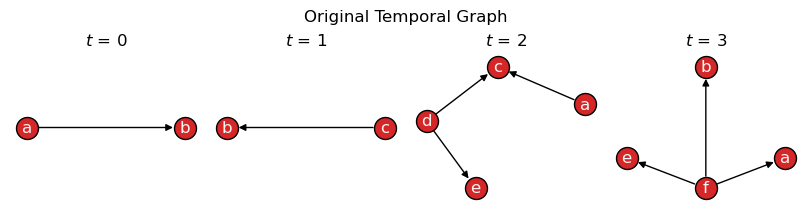
Propagate snapshots

Suppose connections should be instead treated as long-lasting, with future snapshots maintaining past observed data. The propagate_snapshots() function allows to merge previous snapshots forward or backward in time. New nodes and edges for each snapshot are here highlighted in green:

>>> TG = tx.temporal_graph(directed=True)
>>>
>>> TG.add_edge("a", "b", time=0)
>>> TG.add_edge("c", "b", time=1)
>>> TG.add_edge("d", "c", time=2)
>>> TG.add_edge("d", "e", time=2)
>>> TG.add_edge("a", "c", time=2)
>>> TG.add_edge("f", "e", time=3)
>>> TG.add_edge("f", "a", time=3)
>>> TG.add_edge("f", "b", time=3)
>>>
>>> TG = TG.slice(attr="time")
>>>
>>> tx.draw(TG, figsize=(8,2), layout="kamada_kawai", suptitle="Original Temporal Graph")

>>> TG_prop = tx.propagate_snapshots(TG, method="ffill")
>>>
>>> temporal_node_color = [
>>>     ["green" if TG_prop.index_node(n)[0] == t else "tab:red"
>>>      for n in G.nodes()] for t, G in enumerate(TG_prop)]
>>>
>>> temporal_edge_color = [
>>>     ["tab:green" if TG_prop.index_edge((n1, n2))[0] == t else "black"
>>>      for n1, n2 in G.edges()] for t, G in enumerate(TG_prop)]
>>>
>>> tx.draw(TG_prop, figsize=(8, 2), layout="kamada_kawai",
>>>         temporal_node_color=temporal_node_color,
>>>         temporal_edge_color=temporal_edge_color,
>>>         suptitle="Propagated Temporal Graph (ffill)")

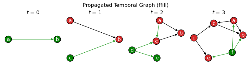
This allows to model scenarios where connections persist over time until removed, which may be useful for the purposes of analyzing and simulating spreading processes, among other applications.

Save and load data

Temporal graphs may be read from or written to a file using read_graph() and write_graph():

>>> tx.write_graph(TG, "temporal-graph.graphml.zip")
>>> TG = tx.read_graph("temporal-graph.graphml.zip")

Supported formats are the same as those in NetworkX and depend on the version installed.

See also

The read and write documentation from NetworkX for a list of supported graph formats.

Inherited methods

Any methods available from a NetworkX graph can be called directly from a TemporalGraph object. For example, the familiar methods below transform edges in the graph into directed or undirected:

>>> TG.to_undirected()

<networkx_temporal.classes.graph.TemporalGraph at 0x7f13dcde4dd0>

>>> TG.to_directed()

<networkx_temporal.classes.digraph.TemporalDiGraph at 0x7f13dcdccdd0>

Note that both methods return new objects when called, so the original graph remains unchanged.

See also

The NetworkX documentation for a list of methods inherited by a TemporalGraph object.

Utility functions

Utility functions for temporal graphs are available in the ~networkx_temporal.utils module.

>>> TG = tx.temporal_graph(multigraph=False)
>>>
>>> TG.add_node("a", group=0)
>>> TG.add_node("b", group=1)
>>> TG.add_node("c", group=1)
>>> TG.add_node("d")
>>>
>>> TG.add_edge("a", "b", time=0)
>>> TG.add_edge("b", "c", time=0)
>>> TG.add_edge("a", "d", time=1)
>>>
>>> print(TG)

TemporalGraph (t=1) with 4 nodes and 3 edges

Node and edge attributes

Obtaining node and edge attributes across snapshots:

>>> tx.get_node_attributes(TG, "group")

[{'a': 0, 'b': 1, 'c': 1, 'd': nan}]

>>> tx.get_edge_attributes(TG, "time")

[{('a', 'b'): 0, ('a', 'd'): 1, ('b', 'c'): 0}]

Partition node and edge sets

Partition nodes and edges based on their attribute values per snapshot:

>>> tx.partition_nodes(TG, "group", index=True, default="unknown")

[{0: ['a'], 1: ['b', 'c'], 'unknown': ['d']}]

>>> tx.partition_nodes(TG, "group", index=False)

[[['a'], ['c', 'b'], ['d']]]

>>> tx.partition_edges(TG, "time")

[{0: [('a', 'b'), ('b', 'c')], 1: [('a', 'd')]}]

Mapping node and edge attributes

Mapping edge-level time to nodes, or node-level group to edges:

>>> tx.map_edge_attr_to_nodes(TG, "time", unique=True)

[{'a': [0, 1], 'b': [0, 0], 'c': [0], 'd': [1]}]

>>> tx.map_node_attr_to_edges(TG, "group", origin="source")

[{('a', 'b'): 0, ('a', 'd'): 0, ('b', 'c'): 1}]

Similarity of node and edge sets

Obtaining a Jaccard similarity matrix (intersection over union) of node sets over time:

>>> snapshots = TG.slice(attr="time")
>>> tx.temporal_node_matrix(snapshots, method="jaccard")

[[1.0, 0.25], [0.25, 1.0]]

See also

The Algorithms and metrics → Temporal evolution examples with similarity matrices.