See also
All examples in this guide are also available as an interactive Jupyter notebook (open on Colab).
Community detection
Community detection is a fundamental task in network analysis. This simple example demonstrates how a network’s temporal dynamics can overall benefit the detection of its mesoscale structures.
Generate graph
As a toy graph, let’s use the simplest Stochastic Block Model to generate 4 snapshots, in which each of the 5 clusters of 5 nodes each continuously mix over time (decreasing assortativity):
>>> import networkx as nx
>>> import networkx_temporal as tx
>>>
>>> nodes = 5       # Number of nodes in each cluster.
>>> clusters = 5    # Number of clusters/communities.
>>> snapshots = 4   # Temporal graphs to generate.
>>>
>>> p = .9          # High initial probability of within-community edges.
>>> q = .1          # Low initial probability of inter-community edges.
>>> rate = .125     # Change in within- and inter-community edges over time.
>>>
>>> TG = tx.from_snapshots([
>>>     nx.stochastic_block_model(
>>>         sizes=[nodes]*clusters,
>>>         p=tx.generate_block_matrix(clusters, p=p-(t*rate), q=q+(t*rate)),
>>>         seed=10
>>>     )
>>>     for t in range(snapshots)
>>> ])
>>>
>>> print(TG)
Let’s plot the graphs, with colors representing communities and within-community edges:
>>> import matplotlib.pyplot as plt
>>> colors = plt.cm.tab10.colors
>>>
>>> def get_edge_color(edges, node_color):
>>>     edge_color = []
>>>     for u, v in edges:
>>>         if node_color[u] == node_color[v]:
>>>             edge_color.append(node_color[u])  # Within-community edge.
>>>         else:
>>>             edge_color.append((0, 0, 0, .25))  # Inter-community edge.
>>>     return edge_color
>>>
>>> # Node positions.
>>> pos = nx.circular_layout(TG.to_static())
>>>
>>> # Node options for all graphs; colorize nodes by block/community.
>>> node_color = [colors[x % len(colors)] for n, x in TG[0].nodes(data="block")]
>>>
>>> # Plot snapshots with community ground truths.
>>> tx.draw(
>>>     TG,
>>>     pos=pos,
>>>     figsize=(12, 3.5),
>>>     node_size=300,
>>>     node_color=node_color,
>>>     edge_color=(0, 0, 0, .3),
>>>     suptitle="Ground truths")
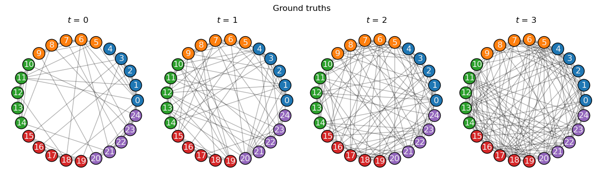
We see that all snapshots are generated with the same community structure, but varying degrees of assortativity. Let’s try to retrieve the ground truths using a simple community detection algorithm.
See also
The dynamic_stochastic_block_model()
function for graphs with time-evolving communities.
Modularity optimization
The leidenalg [1] package implements optimization algorithms for community detection that may be applied on snapshot-based temporal graphs, allowing to better capture their underlying structure.
>>> import leidenalg as la
Attention
Optimization algorithms may help with descriptive or exploratory tasks and post-hoc network analysis, but lack statistical rigor for inferential purposes. See Peixoto (2021) [2] for a discussion.
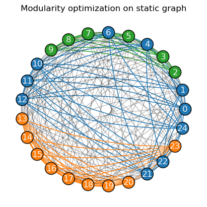
Optimizating static modularity
Let’s start by considering the network as a single static graph, ignoring its temporal information.
We can observe that, depending on the initial node community assignments (e.g., with seed=0 below),
modularity
fails to retrieve the true communities (ground truths) in the network:
>>> membership = la.find_partition(
>>>     TG.to_static("igraph"),
>>>     la.ModularityVertexPartition,
>>>     n_iterations=-1,
>>>     seed=0,
>>> )
>>>
>>> node_color = [colors[x % len(colors)] for x in membership.membership]
>>>
>>> tx.draw(
>>>     TG.to_static(),
>>>     pos=pos,
>>>     figsize=(4, 4),
>>>     node_size=300,
>>>     node_color=node_color,
>>>     edge_color=get_edge_color(TG.to_static().edges(), node_color),
>>>     connectionstyle="arc3,rad=0.1",
>>>     suptitle="Modularity optimization on static graph")
Next, let’s try considering the network’s temporal information to see if we can improve the results.
Running the same algorithm separately on each of the generated snapshots retrieves the correct clusters only on the first graph (\(t=0\)). In addition, community indices (represented by their colors) are not fixed over snapshots, which makes it harder to track their mesoscale dynamics:
>>> snapshot_membership = [
>>>     la.find_partition(
>>>         TG[t:t+1].to_static("igraph"),
>>>         la.ModularityVertexPartition,
>>>         n_iterations=-1,
>>>         seed=0
>>>     ).membership
>>>     for t in range(len(TG))
>>> ]
>>>
>>> temporal_node_color = [
>>>     [colors[m] for m in snapshot_membership[t]]
>>>     for t in range(len(TG))
>>> ]
>>>
>>> tx.draw(
>>>     TG,
>>>     pos=pos,
>>>     figsize=(12, 3.5),
>>>     node_size=300,
>>>     temporal_node_color=temporal_node_color,
>>>     temporal_edge_color=[
>>>         get_edge_color(G.edges(), temporal_node_color[t])
>>>         for t, G in enumerate(TG)
>>>     ],
>>>     connectionstyle="arc3,rad=0.1",
>>>     suptitle="Modularity optimization on graph snapshots")
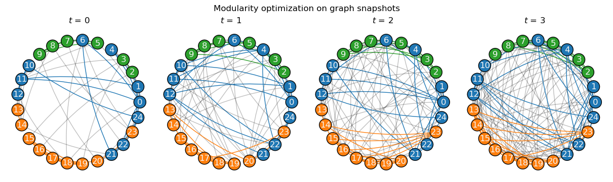
This is partly due to modularity optimization expecting an assortative community structure, while the network grew more disassortative over time. Not only the results of later snapshots are here suboptimal, but the varying community indices increase the complexity of their temporal analysis.
Optimizing multislice modularity
Considering snapshots as layers (slices) of a multiplex graph, with interslice edges coupling temporal node copies, is one way of employing modularity optimization on dynamic graphs, which may help to better capture their mesoscale structures [3]. This example uses the same algorithm as before:
>>> multislice_membership, improvement = la.find_partition_temporal(
>>>     TG.to_snapshots("igraph"),
>>>     la.ModularityVertexPartition,
>>>     interslice_weight=1.0,
>>>     n_iterations=-1,
>>>     seed=0,
>>>     vertex_id_attr="_nx_name"
>>> )
>>>
>>> temporal_node_color = [
>>>     [colors[m] for m in multislice_membership[t]]
>>>     for t in range(len(TG))
>>> ]
>>>
>>> tx.draw(
>>>     TG,
>>>     pos=pos,
>>>     figsize=(12, 3.5),
>>>     node_size=300,
>>>     temporal_node_color=temporal_node_color,
>>>     temporal_edge_color=[
>>>         get_edge_color(G.edges(), temporal_node_color[t])
>>>         for t, G in enumerate(TG)
>>>     ],
>>>     connectionstyle="arc3,rad=0.1",
>>>     suptitle="Modularity optimization on multislice graph")
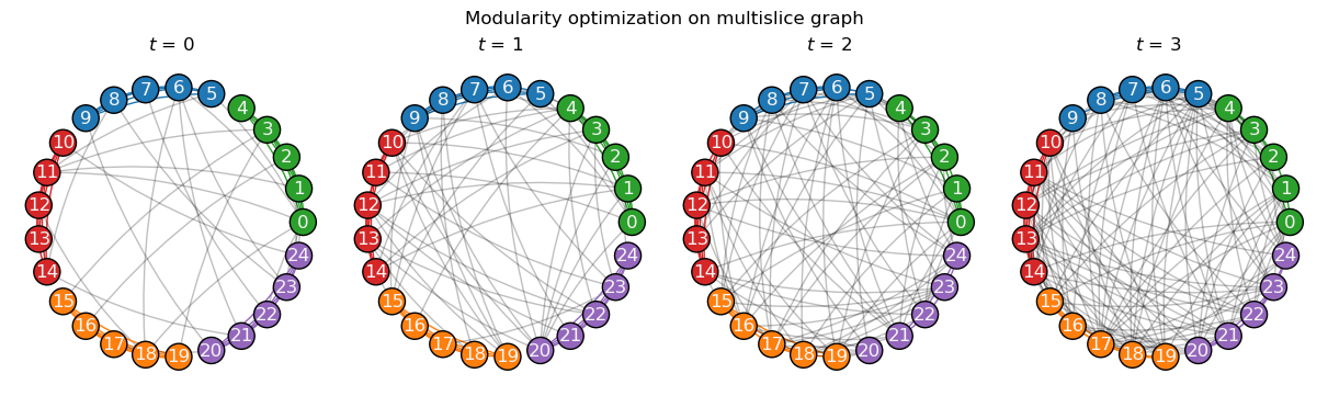
Simply considering the network’s temporal dimension allows modularity optimization to correctly retrieve the ground truths in the network, while maintaining the community indices fixed over time.
Evaluating community structures
We may now compute the modularity for different partitionings and optimization strategies. Let’s compare the values obtained considering static, snapshot, and multislice graph optimization:
>>> modularity = ("Static", "Snapshot", "Multislice")
>>> static_membership = dict(enumerate(membership.membership))  # Static assignments.
>>> partitions = (static_membership, snapshot_membership, multislice_membership)
>>>
>>> for m, assignments in zip(modularity, partitions):
>>>    Q = tx.modularity(TG, assignments)
>>>    mean = sum(Q) / len(Q)
>>>    Q = [round(q, 3) for q in Q]
>>>    print(f"{m}: Q = {Q} (mean: {mean:.3f})")

Static: Q = [0.142, 0.132, 0.078, 0.018] (mean: 0.093)
Snapshot: Q = [0.451, 0.268, 0.182, 0.132] (mean: 0.258)
Multislice: Q = [0.451, 0.26, 0.089, 0.019] (mean: 0.205)
Snapshot-based optimization of modularity returned values of \(Q\) that are higher than those obtained by optimizing it on the static or multislice graphs, but they do not correspond to the ground truths. This illustrates how modularity optimization may yield misleading results when the assumptions of the quality function are not met by the network structure, as in this case.
Note
The same observation can be made for conductance [4], where lower values correspond to more tight-knit communities, with comparatively fewer connections to the rest of the network:
>>> for m, assignments in zip(optimization, partitions):
>>>    conductance = tx.conductance(TG, assignments)
>>>    mean = sum(conductance) / len(conductance)
>>>    conductance = [round(c, 3) for c in conductance]
>>>    print(f"{m}: C = {conductance} (mean: {mean:.3f})")

Static: C = [0.517, 0.533, 0.587, 0.641] (mean: 0.569)
Snapshot: C = [0.344, 0.493, 0.569, 0.536] (mean: 0.486)
Multislice: C = [0.344, 0.532, 0.71, 0.78] (mean: 0.591)
We see how the assumption that communities are assortative structures leads to suboptimal results as it is not shared by this network, which becomes increasingly disassortative over time.
Time-aware quality functions
The multislice_modularity() extension of the static metric
introduces [3] interslice edges connecting temporal node copies, with the goal of better capturing
the quality of temporal community structures. We can compute the multislice modularity \(Q_{ms}\)
for all partitionings:
>>> for m, assignments in zip(optimization, partitions):
>>>     Q_ms = tx.multislice_modularity(TG, assignments, interslice_weight=1)
>>>     print(f"{m}: multislice Q = {Q_ms:.3f}")

Static: multislice Q = 0.075
Snapshot: multislice Q = 0.027
Multislice: multislice Q = 0.076
In this case, the highest value obtained with Leiden optimization corresponds to the ground truth communities. A better description of the network is achieved by considering its temporal dimension, showcasing how time-aware quality functions may improve community detection tasks, even for greedy optimization approaches aiming at a descriptive analysis of the graph.
Mixed-membership communities
Consider the following graph with two assortative communities connected by a bridge node \(d\):
>>> TG = tx.TemporalGraph()
>>> G = TG[0]
>>> G.add_edges_from([
>>>     ("a", "b"), ("b", "c"), ('c', "a"), ("d", "a"),
>>>     ("e", "f"), ("f", "g"), ("g", "e"), ("d", "e"),
>>> ])
>>> tx.draw(G, layout="spring", node_color=list("rrrbggg"))
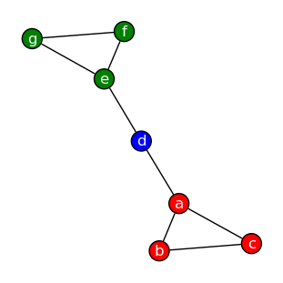
The modularity \(Q\) of a partitioning with node \(d\) in neither community corresponds to:
>>> community_vector = [0, 0, 0,  1 , 2, 2, 2]
>>> tx.modularity(G, community_vector)

0.3515625
If considered to be in either one of the communities, it yields a slightly higher value of \(Q\):
>>> community_vector = [0, 0, 0,  0 , 1, 1, 1]
>>> tx.modularity(G, community_vector)

0.3671875
The spectral_modularity() function implements support for
sparse adjacency matrices and mixed-memberships, where nodes may belong to multiple clusters with
different weights. For example, a high increase in modularity is achieved by considering node \(d\)
in both communities \([0, 1]\):
>>> community_matrix = tx.community_matrix_from_vector(community_vector)
>>> community_matrix[3] = [1, 1]  # Assign node 'd' to both communities 1 and 2.
>>> community_matrix

array([[1., 0.],
       [1., 0.],
       [1., 0.],
       [1., 1.],   # <-- Node 'd' in both communities.
       [0., 1.],
       [0., 1.],
       [0., 1.]])
>>> tx.spectral_modularity(G, community_matrix)
>>> # tx.modularity(G, community_matrix, spectral=True)

0.49375
This suggests algorithms that consider both mixed and dynamic community assignments are more fitting choices to graphs in which nodes should not be restricted to a single community, including greedy optimization approaches, such as algorithms using modularity as a quality function.
References